Rail network

The rail network is the most complex network within the project.

The network can be constructed from:

• NARN data

• Intermodal terminal data

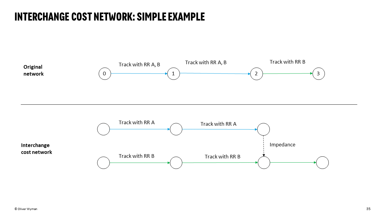
But the NARN data alone is insufficient to construct a “realistic” rail network because it does not account for interchange costs among operators. To do so, we need to examine the railroad owners and railroad operators with trackage rights on each edge.

Given each edge’s set of owner/operators, we can create subgraphs of the entire NARN graph by owner/operator (one subgraph for each operator) and join the subgraphs with “impedance” edges that represent interchange “costs.”

These are accomplished through:

ireiat.data_pipeline.assets.rail_network.impedance._generate_impedances(g: Graph, separation_attribute='owners') → set[tuple[str, tuple[float, float], str, tuple[float, float]]]

Given a graph with a separation_attribute on each edge, determine the impedance edges that would be needed to join subgraphs that were created from unique values of the separation attribute. For example, if a graph of 0 -> 1 -> 2 had ‘owners’ ‘A’ on the first edge and ‘B’ on the second edge (along with origin and destination coords for each edge), this method would return {(‘A’, destination_coords, ‘B’, origin_coords)} given that a graph split by owner would be A graph: 0->1 and B graph: 1->2 and there would be an impedance edge between ‘A1’ and ‘B1’ (with appropriate coordinates returned).

Parameters:

• g – graph to generate impedance edges from

• separation_attribute – string identifer on the graph edges

Returns:

Set of tuples of impedance graph edges

ireiat.data_pipeline.assets.rail_network.impedance._generate_subgraphs(g: Graph, separation_attribute: str = 'owners') → Dict[str, Graph]

Returns subgraphs by unique entries in the separation_attribute for the graph. Returned subgraphs have an ‘original_idx’ field with the format {X}{Y}, where X is the separation_attribute string and Y is the original vertex index. E.g. 0->1 (Graph A) would have [‘A0’,’A1’] vertex attributes

Additionally, each subgraph’s separation_attribute now takes the string of the attribute value to which the subgraph belongs. E.g. Graph with 0->1 (separation_attribute={‘A’,’B’} would have two graphs returned, each with separation_attribute=’A’ or separation_attribute=’B’.

Parameters:

g – graph to separate by a given attribute

Returns:

Dict of subgraphs, keyed by unique separation attribute values

ireiat.data_pipeline.assets.rail_network.impedance.generate_impedance_graph(g: Graph, separation_attribute='owners', config: RailImpedanceConfig | None = None) → Graph

Given a graph whose edges all contain separation_attribute, return an “exploded” graph with impedances edges between vertices that have different values of the separation attribute. See the detailed test cases for how this method is intended to function.

Parameters:

• g – iGraph with separation_attribute of type Set

• separation_attribute – string identifying the attribute

• config – rail configuration when running the data pipeline

Returns:

an exploded graph with impedance edges

ireiat.data_pipeline.assets.rail_network.impedance.generate_impedance_values(impedances: set, config: RailImpedanceConfig | None = None)

Looks up impedance values given the configuration passed, which can be geographic or generic

Note that because there are 900+ owner operators, we only use a subset - but cover ~80% of the relevant rail network edges. Thus, we may not account for some short line interchange fees.

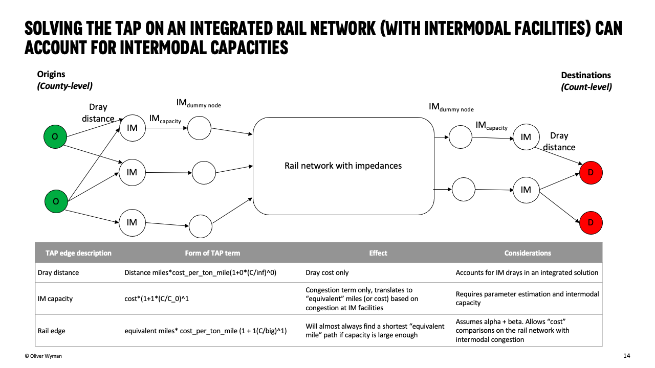
For intermodal facilities, we connect each facility to the impedance graph by adding two new vertices:

1. Intermodal Terminal: Represents the intermodal terminal.

2. Intermodal Dummy Node: Serves as an intermediary connection point for calculating intermodal capacities and costs.

These two nodes are linked by a pair of Intermodal Capacity edges. Each dummy node is then connected to existing rail network nodes based on the terminal’s railroad operators using Rail to Quant or Quant to Rail edges.

After constructing the rail network graph, we prepare it for solving the Traffic Assignment Problem (TAP). This process involves converting the rail network graph into a dataframe that includes essential attributes like speed, free-flow travel time, link capacities, and congestion parameters (alpha and beta) for each link.

Assumptions

1. Speed: Default rail speed is set to 20 miles per hour (mph).

2. Capacity: For intermodal terminal links, the capacity is set to 100,000 tons to reflect the higher throughput of intermodal operations. For standard rail links, the capacity is set to 60,000 tons.

3. Congestion Parameters (Alpha and Beta): For intermodal terminal links, we use alpha = 1 and beta = 1, assuming that congestion is mostly capacity-based and linear. For standard rail links, we use alpha = 0.1 and beta = 3.5 to account for less sensitivity to congestion compared to roads but still reflecting some non-linear impacts.

4. Free-Flow Travel Time (fft): This is calculated as the ratio of link length to speed, representing the time it takes to traverse a link under ideal conditions.